


Next: Robust Averaging
Up: GCX User's Manual
Previous: Multi-Frame and All-Sky Reduction
Contents
Subsections
Noise Modelling
The issue of noise modelling is essential in any photometric endeavour. Measurement values
are next to meaningless if they aren't acompanied by a measure of ther uncertainty.
One can assume that the noise and error modelling only applies to deriving an error figure.
This in true only in extremely simple cases. In general, the noise estimates will also affect
the actual values. For instance, suppose that we use several standards to calibrate a field.
From the noise estimate, we know that one of the standards has a large probable error. Then,
we choose to exclude (or downweight) that value from the solution--this will change the
calibration, and directly affect the result (not just it's noise estimate).
The precision of a measurement denotes the degree to
which different measurements of the same value will yield the same result; it measures the
repeatability of the measurement process. A precise measurement has a small random error.
The accuracy of a measurement denotes the degree to which a measurement result will represent
the true value. The accuracy includes the random error of the measurement, as well as
the systematic error.
Random errors are in a way the worst kind. We have to accept them and take into account, but
they cannot be calculated out. We can try to use better equipment, or more telescope time
and reduce them. On the other hand, since random errors are, well, random in nature (they
don't correlate to anything), we can in principle reduce them to an aribitrarily low level
by averaging a lerge number of measurements.
Systematic errors on the other hand can usually be eliminated (or at least reduced) by
calibration. Systematic errors are not that different from random errors. They differ
fundamentally in the fact the they depend on something. Of course, even random
errors ultimately depend on something. But that something changes incontrollably, and
in a time frame that is short compared to the measurement time scale.
A systematic error can turn into a random error if we have no control over the thing that
the error depends on, or we don't have something to calibrate against. We could treat this
error as ``random'' and try to average many measurements to reduce it, but we have to make
sure that the something that the error depends on has had a change to vary between the
measurements we average, or we won't get very far.
is the ``randomest'' source of random errors. We have no way to
calibrate out noise, but it's features are well understood and relatively easy to model.
One doesn't have a good excuse not to model noise reasonably well.
We will generally talk about ``noise'' when estimating random errors that derive from
an electrical or optical noise source. Once these are combine with
other error sources (like for instance
expected errors of the standards), we will use the term ``error''. Of course, there are two
ways of understanding an error value. If we know what the true value should be, we can talk
about and actual error. If we just consider what error level we can expect, we talk
about an estimated, or expected error.
There are several noise sources in a CCD sensor. We will see that in the end they can
usually be modeled with just two parameters, but we list the main noise contributors
for reference.
- Photon shot noise is the noise associated with the random arrival of photons
at any detector. Shot noise exists because of the discrete nature of light and
electrical charge. The time between photon arrivals is goverened by Poisson
statistics. For a phase-insensitive detector, such as a CCD,
 |
(A.1) |
where  is the signal expressed in electrons. Shot noise is sometimes called
``Poisson noise''.
is the signal expressed in electrons. Shot noise is sometimes called
``Poisson noise''.
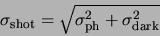
- Output amplifier noise originates in the output amplifier of the sensor.
It consists of two components: thermal (white) noise and flicker noise. Thermal noise
is independent of frequency and has a mild temperature dependence (is proportional to
the square root of the absolute temperature). It fundamentally originates in the thermal
movement of atoms. Flicker noise (or
 noise) is strongly dependent on frequency.
It originates in the existance of long-lived states in the silicon crystal (most notably
``traps'' at the silicon-oxide interface).
noise) is strongly dependent on frequency.
It originates in the existance of long-lived states in the silicon crystal (most notably
``traps'' at the silicon-oxide interface).
For a given readout configuration and speed, these noise sources contribute a constant
level, that is also independant of the signal level, usually called the readout noise.
The effect of read noise can be reduced by increasing the
time in which the sensor is read out. There is a limit to that, as
flicker noise will begin to kick in. For some cameras, one has the option of trading readout
speed for a decrease in readout noise.
- Camera noise. Thermal and flicker noise are also generated in
the camera electronics. the noise level will be independent on the signal.
While the camera designer needs to make a distiction between the
various noise sources, for a given camera, noise originating in the camera and the ccd
amplifier are indistinguishable.
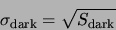
- Dark current noise. Even in the absence of light, electron-hole pairs are generated
inside the sensor. The rate of generation depends exponentially on temperature (typically
doubles every 6-7 degrees). The thermally generated electrons cannot be separated from
photo-generated photons, and obey the same Poisson statistic, so
 |
(A.2) |
We can subtract the average
dark signal, but the shot noise associated with it remains. The level of the dark current
noise depends on temperature and integration time.
- Clock noise. Fast changing clocks on the ccd can also generate spurious charge.
This charge also has a shot noise component associated. However, one cannot read the sensor
without clocking it, so clock noise cannot be discerned from readout noise. The clock noise
is fairly constant for a given camera and readout speed, and independent of the signal level.
Examining the above list, we see that some noise sources are independent of the signal level.
They are: the output amplifier noise, camera noise and clock noise. They can be combined in
a single equivalent noise source. The level of this source is called readout noise, and
is a characteristic of the camera. It can be expressed in electrons, or in the camera output
units (ADU).
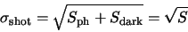
The rest of the noise sources are all shot noise sources. The resulting value will be:
 |
(A.3) |
 |
(A.4) |
 is the total signal from the sensor above bias, expressed in electrons. So to calculate the
shot noise component, we just need to know how many ADUs/electron the camera produces. This
is a constant value, or one of a few constant values for cameras that have different gain
settings. We will use
is the total signal from the sensor above bias, expressed in electrons. So to calculate the
shot noise component, we just need to know how many ADUs/electron the camera produces. This
is a constant value, or one of a few constant values for cameras that have different gain
settings. We will use  to denote this value.
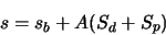
We will now try to model the level of noise in a pixel value. The result of reading one pixel
(excluding noise) is:
 |
(A.5) |
where  is a fixed bias introduced by the camera electronics,
  is the number of
dark electrons, and
is the number of
dark electrons, and  is the number of photo-generated electrons (which is the number
of photons incident on the pixel multiplied by the sensor's quantum efficiency).
is the number of photo-generated electrons (which is the number
of photons incident on the pixel multiplied by the sensor's quantum efficiency).
Now let's calculate the noise associated with this value.
 |
(A.6) |
Where  is the readout noise expressed in ADU, and is the total signal
expressed in electrons. Note that we cannot calculate
the noise if we don't know the bias value. The bias can be determined by reading
frames with zero exposure time (bias frames). These will contribute some read noise though.
By averaging several bias frames, the noise contribution can be reduced. Another approach is
to take the average across a bias frame and use that value for the noise calculation of all
pixels. Except for very non-uniform sensors this approach works well. GCX supports both
ways.
is the readout noise expressed in ADU, and is the total signal
expressed in electrons. Note that we cannot calculate
the noise if we don't know the bias value. The bias can be determined by reading
frames with zero exposure time (bias frames). These will contribute some read noise though.
By averaging several bias frames, the noise contribution can be reduced. Another approach is
to take the average across a bias frame and use that value for the noise calculation of all
pixels. Except for very non-uniform sensors this approach works well. GCX supports both
ways.
Note that a bias frame will only contain readout noise. By calculating the standard
deviation of pixels across the difference between two bias frames we obtain  times the
readout noise.
times the
readout noise.
A common situation is when one subtracts a dark frame, but doesn't use bias frames.
The noise associated with the dark frame is:
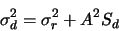 |
(A.7) |
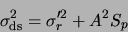
The resulting pixel noise after dark frame subtraction will be:
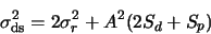 |
(A.8) |
while the signal will be
 |
(A.9) |
Using just the camera noise parameters, we cannot determine the noise anymore.
We have to keep track of the dark subtraction and it's noise effects. We however
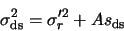
rewrite the dark-subtracted noise equation as follows:
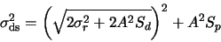 |
(A.10) |
If we use the notation
 , we get:
 |
(A.11) |
This is identical in form to the simple pixel noise equation, except that the true
camera readout noise is replaced by the equivalent read noise  . What's more, the
bias is no longer an issue, as it doesn't appeear in the signal equation anymore. We can
derive the pixel noise from the signal directly, as:
. What's more, the
bias is no longer an issue, as it doesn't appeear in the signal equation anymore. We can
derive the pixel noise from the signal directly, as:
 |
(A.12) |
The same parameters, and are sufficient to describe the noise in the
dark-subtracted frame.
To flat-field a frame, we divide the dark-subtracted pixel value  by the flat field
value
by the flat field
value  . The noise of the flat field is
  . The resulting signal value is
 |
(A.13) |
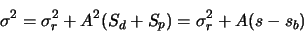
If we neglect second-order noise terms, the noise of the flat-fielded, dark subtracted pixel
is:
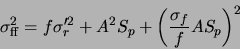 |
(A.14) |
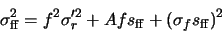 |
(A.15) |
The problem with this result is that f is not constant across the frame. So in general, the noise
of a flat-fielded frame cannot be described by a small number of parameters. In many cases though,
doesn't vary too much across the frame. We can then use it's average value,  for the noise calculation. This is the approach taken by the program.
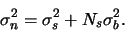
We can identify the previous noise parameters,
 and
and
 . For specifing the
effect of the flat-fielding, we introduce a new parameter,
.
. For specifing the
effect of the flat-fielding, we introduce a new parameter,
.
Without reducing generality, we can arrange for
 . This means that the
average values on the frames don't change with the flatfielding operation, and is a common
choice.
. This means that the
average values on the frames don't change with the flatfielding operation, and is a common
choice.
In this case, and aren't affected by the flatfielding operation, while the
third noise parameter becomes
 , which is the reciprocal of the SNR of
the flat field.
, which is the reciprocal of the SNR of
the flat field.
GCX models the noise of each pixel in the frame by four parameters: , ,
and
 . The noise function
  of each pixel
is:
of each pixel
is:
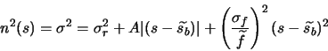 |
(A.16) |
comes from the RDNOISE field in the frame header. is the
reciprocal of the value of the ELADU field.
comes from
FLNOISE, while
comes from DCBIAS.
Every time frames are processed
(dark and bias subtracted, flatfielded, scaled etc), the noise parameters are updated.
Once we know the noise of each pixel, deriving the expected error of an instrumental magnitude
is straightforward. Let  be the number of pixels in the sky annulus, and
  the level
of each pixel. The noise of the sky estimate is:A.1
the level
of each pixel. The noise of the sky estimate is:A.1
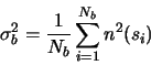 |
(A.17) |
Now let  be the number of pixels in the central aperture. The noise from these pixels is:
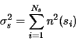 |
(A.18) |
The total noise after sky subtraction will be:
 |
(A.19) |
The program keeps track and reports separately the photon shot noise, the sky noise,
the read noise contribution and the scintillation noise.
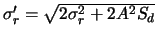
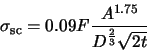
Scintillation is an atmospheric effect, which results in a random variation of the
received flux from a star. We use the following formula for scintillation noise:
 |
(A.20) |
Where  is the total flux received from the star, is the airmass of the observation,
 is the telescope aperture in cm, and
  is the integration time. Scintillation varies
widely over time, so the above is just an estimate.
is the integration time. Scintillation varies
widely over time, so the above is just an estimate.
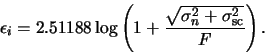
Finally, we can calculate the expected error of the instrumental magnitude as
 |
(A.21) |
Next: Robust Averaging
Up: GCX User's Manual
Previous: Multi-Frame and All-Sky Reduction
Contents
Radu Corlan
2004-12-07